Maximum s-t-Flow and minimum cut

In the vast ocean of combinatorial optimization problems, the Maximum Flow Problem stands out as a challenging and intriguing puzzle with applications spanning across diverse fields. This problem, deeply rooted in network theory, seeks to find the optimal flow of a resource through a network, ultimately illuminating the most efficient path from source to sink. As we delve into the intricacies of this problem, we uncover its significance in fields as varied as transportation, telecommunication, and biology.

Maximum/minimun Flow

Graphs are a common tool for solving various problems, and one way to represent specific network capacities within them is through the concept of flow. This notion of flow is versatile, applicable to scenarios such as determining how much water a pipe can carry or gauging the volume of traffic that can traverse a network like the internet.

In the context of these networks, a maximum flow is achieved when the flow value is either smaller than or equal to the network’s capacity. It’s important to note that a maximum flow can potentially be a blocking flow, although it’s not a mandatory condition. Conversely, the minimum flow is characterized by a nearly zero flow value. This establishes a clear distinction between the maximum and minimum flows, offering a nuanced understanding of the flow dynamics within a network.

Blocking flows

Blocking flows are flows that utilize the entire capacity of the current edge, leaving no room for any additional flow to pass through without surpassing the edge’s capacity limit. In essence, once a blocking flow is in effect, further flow along that path becomes unfeasible without breaching the predefined capacity constraint of the edge.

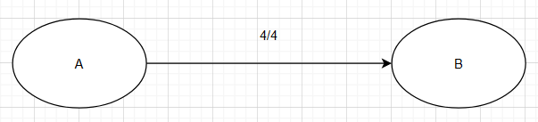
Edge A to B is a blocking flow. There is a flow 4 out of capacity 4.

Augmenting paths

An augmenting path, denoted as p = {s, …, t} in a graph G = (V, E) from vertex s to t (where s, t ∈ V), exists when the flow along path p is less than its capacity. In other words, an augmenting path is present only if there is unused capacity along the path.

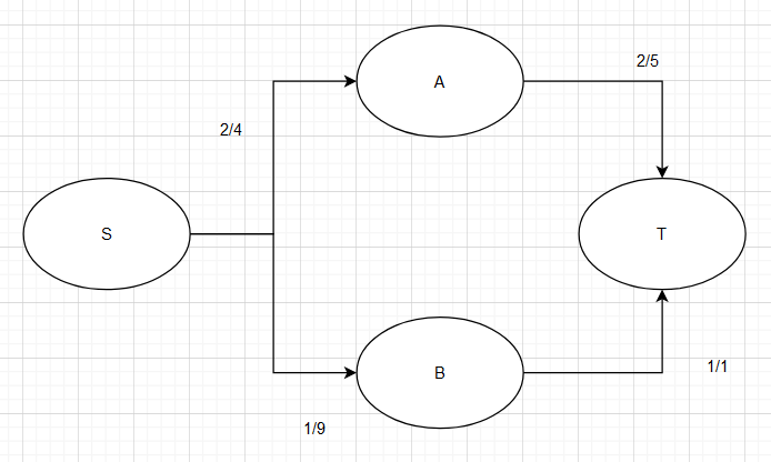
The only possible augmenting path in this graph is p={S,A,T} because there is some spare capacity left.

Side note: The maximum flow here would be 5

Residual graph

TODO

Ford-Fulkerson algorithm

One of the simpler approaches to solving this problem is to consider each augmenting path individually and aggregate the flows, summing them up to determine the maximum flow value. If a particular path leads to a non-augmenting scenario, it is permissible to revert the flow and explore an alternative augmenting path.

proc FFMaxFlow(G=(V,E), s:Node,t:Node)
     f=0
     while ∃path p from s -> t do
          augment f along p
     return f

Runtime of the algorithm is O(|V|*value(f))

Dinitz algorithm

This algorithm shares a similar approach with Ford-Fulkerson. However, rather than simply selecting each augmenting path, it assigns a level to each node, indicating its distance from the sink. After computing the flow, we reassign the levels using Breadth-First Search (BFS). With the updated levels, the flow calculation is repeated iteratively until there are no more paths from the source to the sink.

proc dinitzMaxFlow(G=(V,E), s:Node, t:Node)
     f=0
     while ∃path p from s -> t do
         d=reverseBFS(t)
         L=(V, {(u,v) ∊ E : d(v)=d(u)-1})
         find a blocking b flow in L
         augment f += b
     return f

Following runtimes for the algorithm are known.

Runtime	Notes
O(|V|²*|E|)	Strongly polynomial
O(sqr(|V|*|E|))	On Bipartite graphs
O(|V|*|E|*log|E|)	On dynamic trees

Push-Relable algorithm

This algorithm allows for the creation of excess in nodes, combining functionalities from both Dinitz and Ford-Fulkerson. Begin by setting the source’s level to the total number of available nodes and push the flow to its neighbors. For each node with an excess greater than 0, relabel the node with a higher potential and continue pushing the excess until none remains. If further pushing is not possible, revert the flow to a preceding node, possibly all the way back to the source if needed. Repeat these steps until achieving either a maximum flow or encountering a blocking flow, ensuring that no node has an excess greater than 0 except for the sink.

proc preflowPush(G=(V,E), s: Node, t:Node)
     forall e=(s,v) ∊ E do
        push(e,capacity(e))
     d(s)=n
     d(v)=0 //set the label for all nodes beside s to 0
     while ∃v ∊ V\{s,t} : excees(v) > 0 do
         if ∃e=(v,w) ∊ E : d(w) < d(v) then
            choose some q <= min{excees(v), capacity}
            push(e,q)
         else
            d(v)++

The runtime of this algorithm is denoted here.

Runtime	Notes
O(|V|²*|E|)
O(|V|³)	With FiFo-Queue

Cuts

Consider a pipe system transporting water. If we remove a specific pipe, the overall flow within the system may be altered. Cuts provide a description of the amount of capacity lost by executing such an action, shedding light on the impact of removing a particular component from the system.

Max-Flow = Min-Cut

A proven duality exists between maximum flow and minimum cut. When calculating the maximum flow, the corresponding value of the minimum cut in the residual graph is inherently obtained.

Dynamic programming solution

Moreover, there are alternative feasible solutions for this problem. One option is to employ dynamic programming principles. The concept of dynamic programming has been elucidated in another article on my blog. In this context, I am sharing the solution without delving into the rationale behind this approach, assuming it is already familiar.

Assume we have G=(V,E) with s∊V beeing the source and t∊V beeing the sink. Each node has a capacity c(u,v) and a flow f(u,v) with u,v∊E.

The dynamic approach does look like the following statement.

maximize:
    max(∑f(s,x) - ∑f(u,s)) : (s,x)∊E ⋀ (u,s)∊E

subject to:
    ∀(u,v)∊E   : f(u,v) ≤ c(u,v)
    ∀v∊V\{s,t} : ∑f(s,x) - ∑f(u,s) = 0
    ∀(u,v)∊E   : f(u,v) ≥ 0

human readable solution: maximize the flow out of the sink subtrakted by the flow into the source for all nodes in our graph, meeting the conditions

• The flow must be smaller equals the capacity on this edge
• The flow must be 0 on every node except the source and the sink
• The flow must be greater equals 0

With this conditions its possible to create a dynamic programming solution for the maximum s-t-flow problem.

Sources

Actually for this article I just used my own summary, i made during the semester at my university. I do not have the sources anymore but here are some recomendations for this subject.

https://en.wikipedia.org/wiki/Dynamic_programming (26.1.2024 13:07)

https://www.geeksforgeeks.org/max-flow-problem-introduction/ (26.1.2024 13:15)

https://en.wikipedia.org/wiki/Maximum_flow_problem (26.1.2024 13:16)