Linear programming

In the case of a maximization or minimization problem, it is possible to formulate the problem as a linear program (LP) such that solving it provides a feasible solution, even for NP-hard problems. To achieve this, the problem must be expressed as an LP or integer linear program (ILP), enabling the search for bounds within the solution space. This approach allows for leveraging optimization techniques to find solutions within a computationally manageable framework.

General form

In general, to approach problem-solving using this method, you need to identify a vector in your solution space, denoted as x ∈ R with dimension n, and establish a cost function represented by c. The process involves defining constraints to obtain a feasible solution.

The general form of the problem can be expressed as follows, where the crucial elements are the „maximize/minimize“ directive and the „subject to“ section. This signifies the objective of finding either a maximum or minimum value within certain constraints. The aim is to articulate as many constraints as possible to narrow down the solution space.

maximize/minimize:
    ∑c*x 

subject to:
    x > 0
    ∑c*x = b
    ∑c*x < b : for different c,x,b
    ∑c*x > b : for different c,x,b
    ...

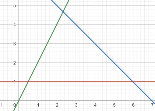
In the general form we need 3 constrains at least. There must be an upper bound, exact bound and a lower bound. The solution space will look like this when having bounds in linear form.

A possible solution space could look like the this graphic if the 3 colored functions represent the boundaries. In this case all feasible solutions are placed inside the triangle with the best solutions beeing placed in the crossing points of the functions.

Canonical form

The canonical form is similar to the general form with difference to the exact bound which does not exist here. We only define the upper bound meaning something like ∑c*x < b and the non negative bound.

maximize/minimize:
    ∑c*x 

subject to:
    x > 0
    ∑c*x < b : for different c,x,b
    ...

Slack form

In this form we only have the exact bound and the non negative bound for the input vector.

maximize/minimize:
    ∑c*x 

subject to:
    x > 0
    ∑c*x = b
    ...

Conversion between forms

=> TODO

Integer linear programming

The ILP problem differs from the LP problem in allowing integer values for the input vector. The important difference between LP and ILP is that LP only allows real numbers and ILP as already mentioned integer valued inputs. Finally ILP is a more general form of LP, as it allows the inclusion of discrete decision variables. E.g if the input vector x ∊ {0,1}

A feasible solution for the ILP is also a solution for LP but if LP has a solution it does not implie that ILP has a solution.

Example of LP and ILP

Assume we have G=(V,E) with s∊V beeing the source and t∊V beeing the sink. Each node has a capacity c(u,v) and a flow f(u,v) with u,v∊E.

maximize:
    max(∑f(s,x) - ∑f(u,s)) : (s,x)∊E ⋀ (u,s)∊E

subject to:
    ∀(u,v)∊E   : f(u,v) ≤ c(u,v)
    ∀v∊V\{s,t} : ∑f(s,x) - ∑f(u,s) = 0
    ∀(u,v)∊E   : f(u,v) ≥ 0

here we have a LP solution of the maximum s-t-flow problem. Generally speaking a LP problem can be defined as a maximizing or a minimizing problem with boundarys giving a smaller solution space.

Infeasible solutions

A suitable example for infeasible solutions is the following lp problem.

maximize:
    x-y
subject to:
    2x+y≤1
    x+y≥2
    x,y≥0

The given example has bounds which make it impossible to find a feasible solution. There is no prove for this as it might be obvious that 2x+y≤1 and x+y≥2 is not possible to hold at the same time when picking any x,y∊R.

Unbounded solutions

Similar to the infeasible solutions there can be unbounded solutions.

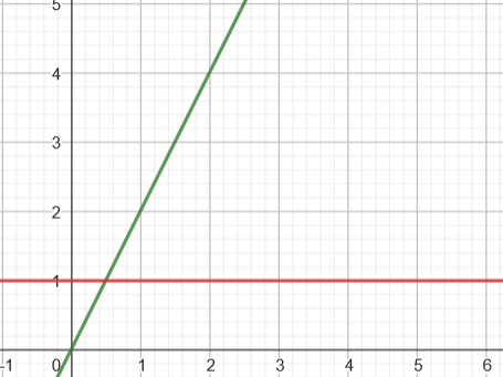
As there is no bound to lim(x) ->∞ it is possible that there is no optimal solution because the solution space is not finite.

Simplex algorithm

The simplex algorithm is one oppertunity to search for the best feaseable solution out of our solution space. Since we know that the best solution vector can be found in a corner area (two or more constrains crossing each other) we just need to check each „corner“ solution and compare it to each other and find the most feaseable solution. Its important to mention that the selected solution is a solution and not the best solution. Reason for that is, that many optimization problems that can be solved with lp or ilp are NP-hard and do not have an optimal solution.

This algorithm might not terminte in the case of an unbounded direction, meaning if there’s no bound we cannot find a optimal solution.

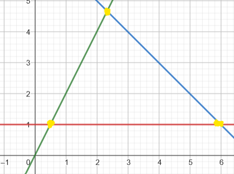
The yellow points denote optimal solutions.

Interior point method

This is another possiblility to find the best solution vector in the solution space. Since the simplex algorithm searchs by searching vectors on the boundarys of our constrains, the interior point method decides by traversing feasible solutions in a elipse form instead of traversing the boundarys.

In theory this is a faster solution compared to the simplex algorithm but in practice this is as fast as the simplex algorithm. More information about this topic are linked in the sources below.

Sources

https://en.wikipedia.org/wiki/Interior-point_method (26.1.2024 17:00)

https://www.cs.carleton.edu/cs_comps/2324/integerLinearPrograming/index.php (26.1.2024 17:15)

https://cs.stackexchange.com/questions/135969/when-lp-solution-is-ilp-solution (26.1.2024 17:19)

https://math.stackexchange.com/questions/176559/lp-relaxation-for-integer-linear-programming-ilp (26.1.2024 17:24)